Motion Classification and Anomaly Detection
Overview
Transportation is the backbone of global commerce. Millions of containers are transported daily via various means, such as ships, trucks, and trains, to destinations worldwide. Ensuring the safe and efficient transit of these containers is a monumental task that requires leveraging modern technology, and TinyML is undoubtedly one of the key solutions.
In this hands-on lab, we will work to solve real-world problems related to transportation. We will develop a Motion Classification and Anomaly Detection system using the XIAOML Kit, the Arduino IDE, and the Edge Impulse Studio. This project will help us understand how containers experience different forces and motions during various phases of transportation, including terrestrial and maritime transit, vertical movement via forklifts, and periods of stationary storage in warehouses.
- Setting up the XIAOML Kit
- Data Collection and Preprocessing
- Building the Motion Classification Model
- Implementing Anomaly Detection
- Real-world Testing and Analysis
By the end of this lab, you’ll have a working prototype that can classify different types of motion and detect anomalies during the transportation of containers. This knowledge can serve as a stepping stone to more advanced projects in the burgeoning field of TinyML, particularly those involving vibration.
Installing the IMU
The XIAOML Kit comes with a built-in LSM6DS3TR-C 6-axis IMU sensor on the expansion board, eliminating the need for external sensor connections. This integrated approach offers a clean and reliable platform for motion-based machine learning applications.
The LSM6DS3TR-C combines a 3-axis accelerometer and 3-axis gyroscope in a single package, connected via I2C to the XIAO ESP32S3 at address 0x6A that provides:
- Accelerometer ranges: ±2/±4/±8/±16 g (we’ll use ±2g by default)
- Gyroscope ranges: ±125/±250/±500/±1000/±2000 dps (we’ll use ±250 dps by default)
- Resolution: 16-bit ADC
- Communication: I2C interface at address 0x6A
- Power: Ultra-low power design
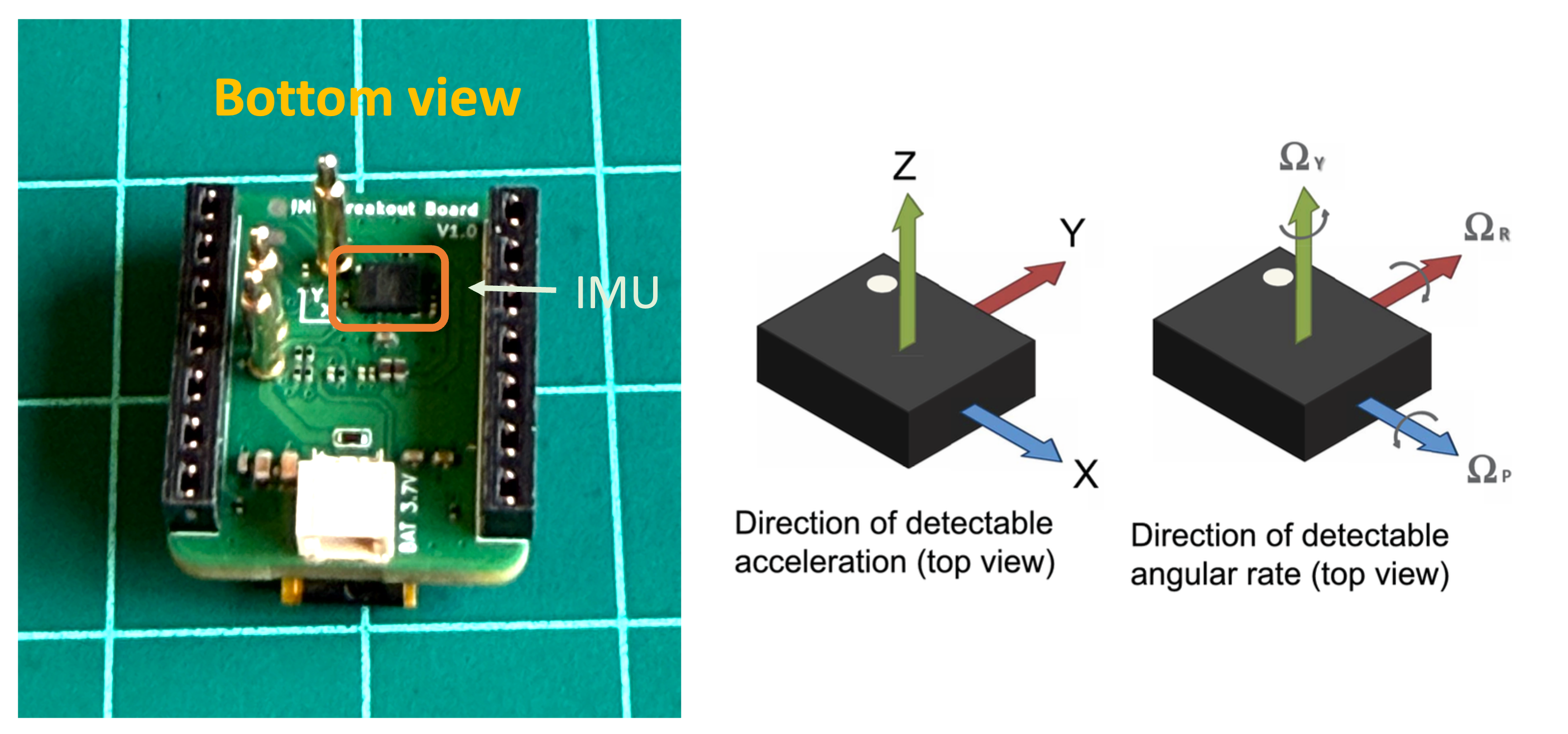
Coordinate System: The sensor operates within a right-handed coordinate system. When looking at the expansion board from the bottom (where you can see the IMU sensor with the point mark):
- X-axis: Points to the right
- Y-axis: Points forward (away from you)
- Z-axis: Points upward (out of the board)
Setting Up the Hardware
Since the XIAOML Kit comes pre-assembled with the expansion board, no additional hardware connections are required. The LSM6DS3TR-C IMU is already properly connected via I2C.
What’s Already Connected:
- LSM6DS3TR-C IMU → I2C (SDA/SCL) → XIAO ESP32S3
- I2C Address: 0x6A
- Power: 3.3V from XIAO ESP32S3
Required Library: You should have the library installed during the Setup. If not, install the Seeed Arduino LSM6DS3 library following the steps:
- Open Arduino IDE Library Manager
- Search for “LSM6DS3”
- Install “Seeed Arduino LSM6DS3” by Seeed Studio
- Important: Do NOT install “Arduino_LSM6DS3 by Arduino” - that’s for different boards!
Testing the IMU Sensor
Let’s start with a simple test to verify the IMU is working correctly. Upload this code to test the sensor:
#include <LSM6DS3.h>
#include <Wire.h>

// Create IMU object using I2C interface
LSM6DS3 myIMU(I2C_MODE, 0x6A);

float accelX, accelY, accelZ;
float gyroX, gyroY, gyroZ;

void setup() {
  Serial.begin(115200);
  while (!Serial) delay(10);

  Serial.println("XIAOML Kit IMU Test");
  Serial.println("LSM6DS3TR-C 6-Axis IMU");
  Serial.println("====================");

  // Initialize the IMU
  if (myIMU.begin() != 0) {
      Serial.println("ERROR: IMU initialization failed!");
      while(1) delay(1000);
  } else {
      Serial.println("✓ IMU initialized successfully");
      Serial.println("Data Format: AccelX,AccelY,AccelZ,"
                    "GyroX,GyroY,GyroZ");
      Serial.println("Units: g-force, degrees/second");
      Serial.println();
  }
}

void loop() {
  // Read accelerometer data (in g-force)
  accelX = myIMU.readFloatAccelX();
  accelY = myIMU.readFloatAccelY();
  accelZ = myIMU.readFloatAccelZ();

  // Read gyroscope data (in degrees per second)
  gyroX = myIMU.readFloatGyroX();
  gyroY = myIMU.readFloatGyroY();
  gyroZ = myIMU.readFloatGyroZ();

  // Print readable format
  Serial.print("Accel (g): X="); Serial.print(accelX, 3);
  Serial.print(" Y="); Serial.print(accelY, 3);
  Serial.print(" Z="); Serial.print(accelZ, 3);
  Serial.print(" | Gyro (°/s): X="); Serial.print(gyroX, 2);
  Serial.print(" Y="); Serial.print(gyroY, 2);
  Serial.print(" Z="); Serial.println(gyroZ, 2);

  delay(100); // 10 Hz update rate
}
When the kit is resting flat on a table, you should see:
- Z-axis acceleration around +1.0g (gravity)
- X and Y acceleration near 0.0g
- All gyroscope values near 0.0°/s
Move the kit around to see the values change accordingly.
The TinyML Motion Classification Project
We will simulate container (or, more accurately, package) transportation through various scenarios to make this tutorial more relatable and practical.
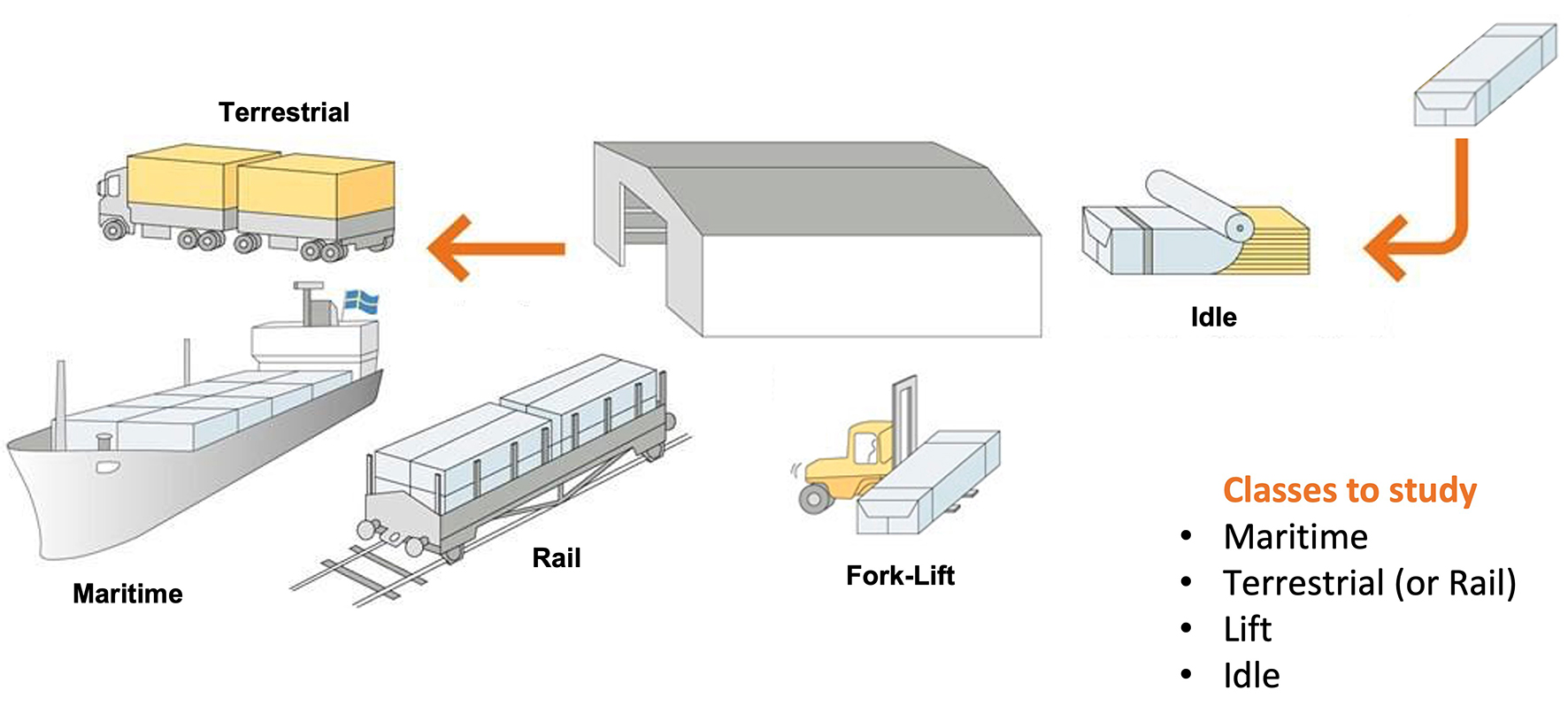
Using the accelerometer of the XIAOML Kit, we’ll capture motion data by manually simulating the conditions of:
- Maritime (pallets on boats) - Movement in all axes with wave-like patterns
- Terrestrial (pallets on trucks/trains) - Primarily horizontal movement
- Lift (pallets being moved by forklift) - Primarily vertical movement
- Idle (pallets in storage) - Minimal movement
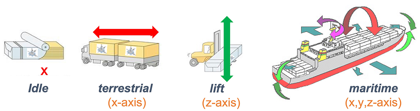
From the above image, we can define for our simulation that primarily horizontal movements (\(x\) or \(y\) axis) should be associated with the “Terrestrial class.” Vertical movements (\(z\)-axis) with the “Lift Class,” no activity with the “Idle class,” and movement on all three axes to Maritime class.
Data Collection
For data collection, we have several options available. In a real-world scenario, we can have our device, for example, connected directly to one container, and the collected data stored in a file (for example, CSV) on an SD card. Data can also be sent remotely to a nearby repository, such as a mobile phone, using Wi-Fi or Bluetooth (as demonstrated in this project: Sensor DataLogger). Once your dataset is collected and stored as a .CSV file, it can be uploaded to the Studio using the CSV Wizard tool.
In this video, you can learn alternative ways to send data to the Edge Impulse Studio.
Preparing the Data Collection Code
In this lab, we will connect the Kit directly to the Edge Impulse Studio, which will also be used for data pre-processing, model training, testing, and deployment.
For data collection, we should first connect the Kit to Edge Impulse Studio, which will also be used for data pre-processing, model training, testing, and deployment.
Follow the instructions here to install Node.js and Edge Impulse CLI on your computer.
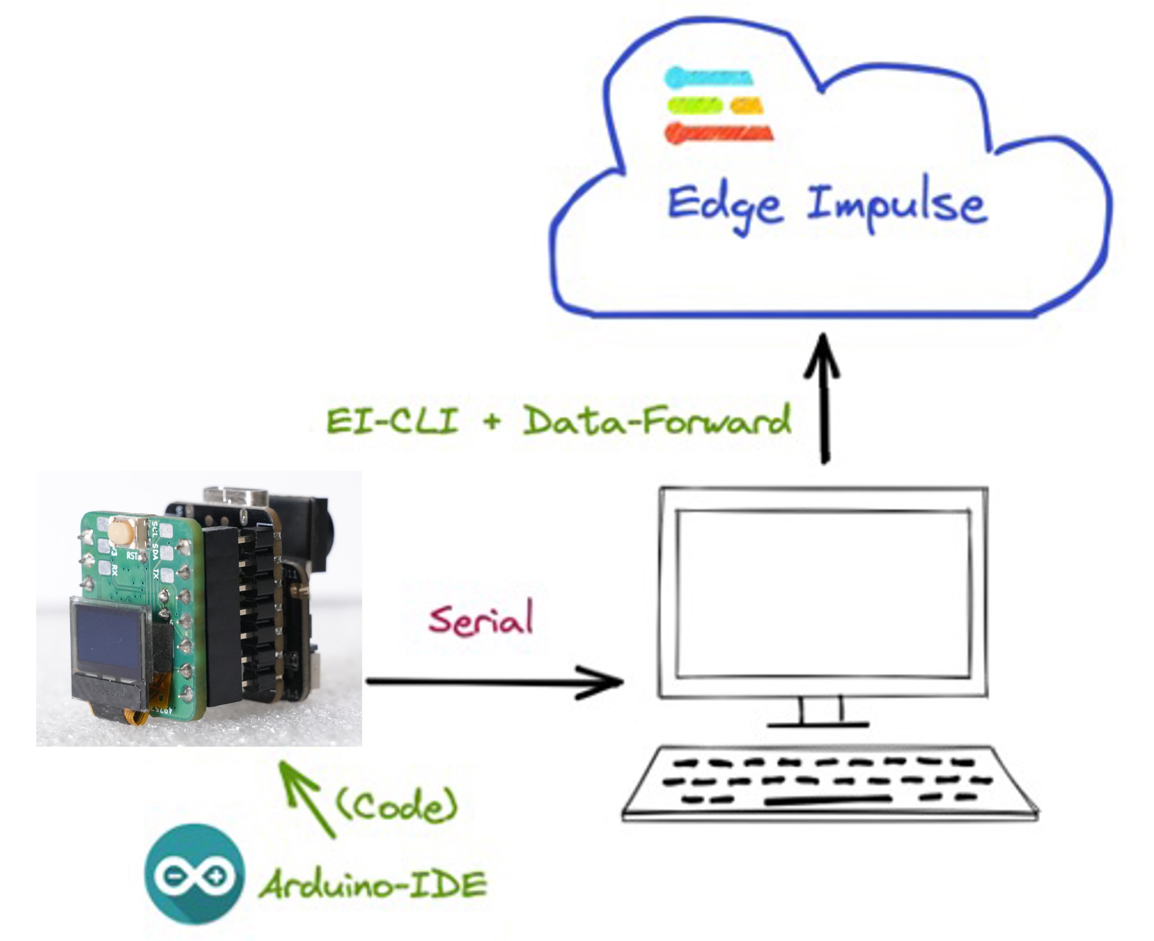
Once the XIAOML Kit is not a fully supported development board by Edge Impulse, we should, for example, use the CLI Data Forwarder to capture data from our sensor and send it to the Studio, as shown in this diagram:
We’ll modify our test code to output data in a format suitable for Edge Impulse:
#include <LSM6DS3.h>
#include <Wire.h>
#define FREQUENCY_HZ 50
#define INTERVAL_MS (1000 / (FREQUENCY_HZ + 1))
LSM6DS3 myIMU(I2C_MODE, 0x6A);
static unsigned long last_interval_ms = 0;
void setup() {
Serial.begin(115200);
while (!Serial) delay(10);
Serial.println("XIAOML Kit - Motion Data Collection");
Serial.println("LSM6DS3TR-C IMU Sensor");
// Initialize IMU
if (myIMU.begin() != 0) {
Serial.println("ERROR: IMU initialization failed!");
while(1) delay(1000);
}
delay(2000);
Serial.println("Starting data collection in 3 seconds...");
delay(3000);
}
void loop() {
if (millis() > last_interval_ms + INTERVAL_MS) {
last_interval_ms = millis();
// Read accelerometer data
float ax = myIMU.readFloatAccelX();
float ay = myIMU.readFloatAccelY();
float az = myIMU.readFloatAccelZ();
// Convert to m/s² (multiply by 9.81)
float ax_ms2 = ax * 9.81;
float ay_ms2 = ay * 9.81;
float az_ms2 = az * 9.81;
// Output in Edge Impulse format
Serial.print(ax_ms2);
Serial.print("\t");
Serial.print(ay_ms2);
Serial.print("\t");
Serial.println(az_ms2);
}
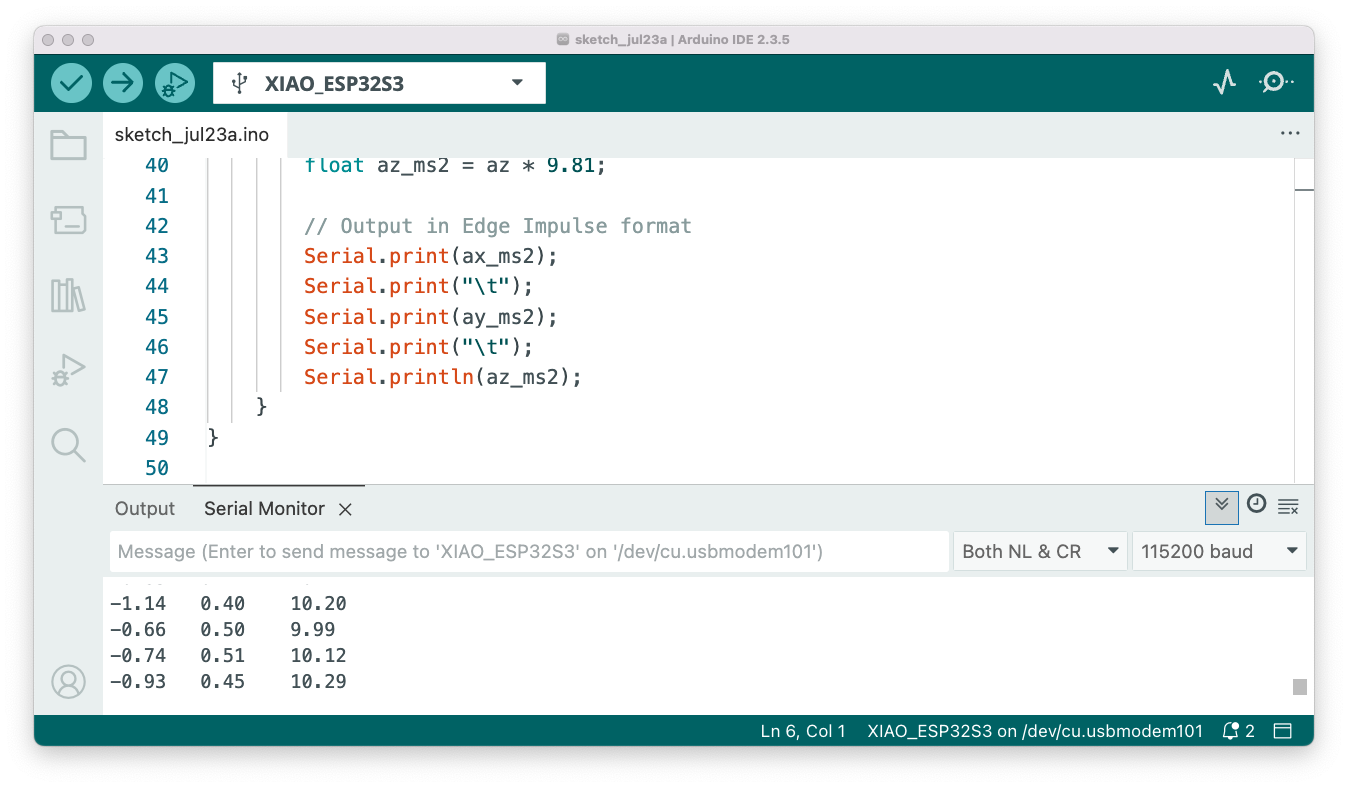
}Upload the code to the Arduino IDE. We should see the accelerometer values (converted to m/s²) at the Serial Monitor:
Keep the code running, but turn off the Serial Monitor. The data generated by the Kit will be sent to the Edge Impulse Studio via Serial Connection.
Connecting to Edge Impulse for Data Collection
Create an Edge Impulse Project - Go to Edge Impulse Studio and create a new project - Choose a descriptive name (keep under 63 characters for Arduino library compatibility)

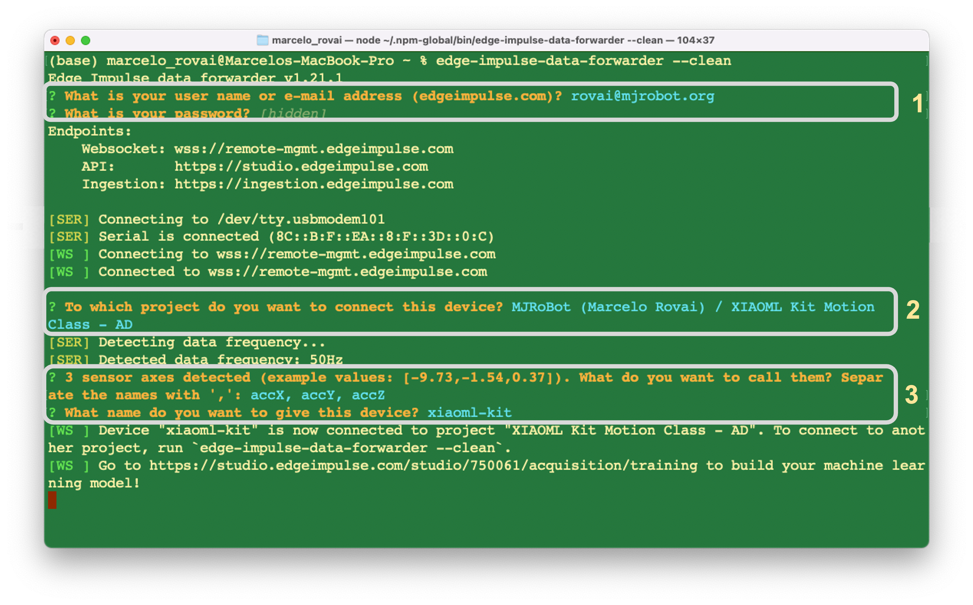
Set up CLI Data Forwarder - Install Edge Impulse CLI on your computer - Confirm that the XIAOML Kit is connected to the computer, the code is running and the Serial Monitor is OFF, otherwise we can get an error. - On the Computer Terminal, run: edge-impulse-data-forwarder --clean - Enter your Edge Impulse credentials - Select your project and configure device settings
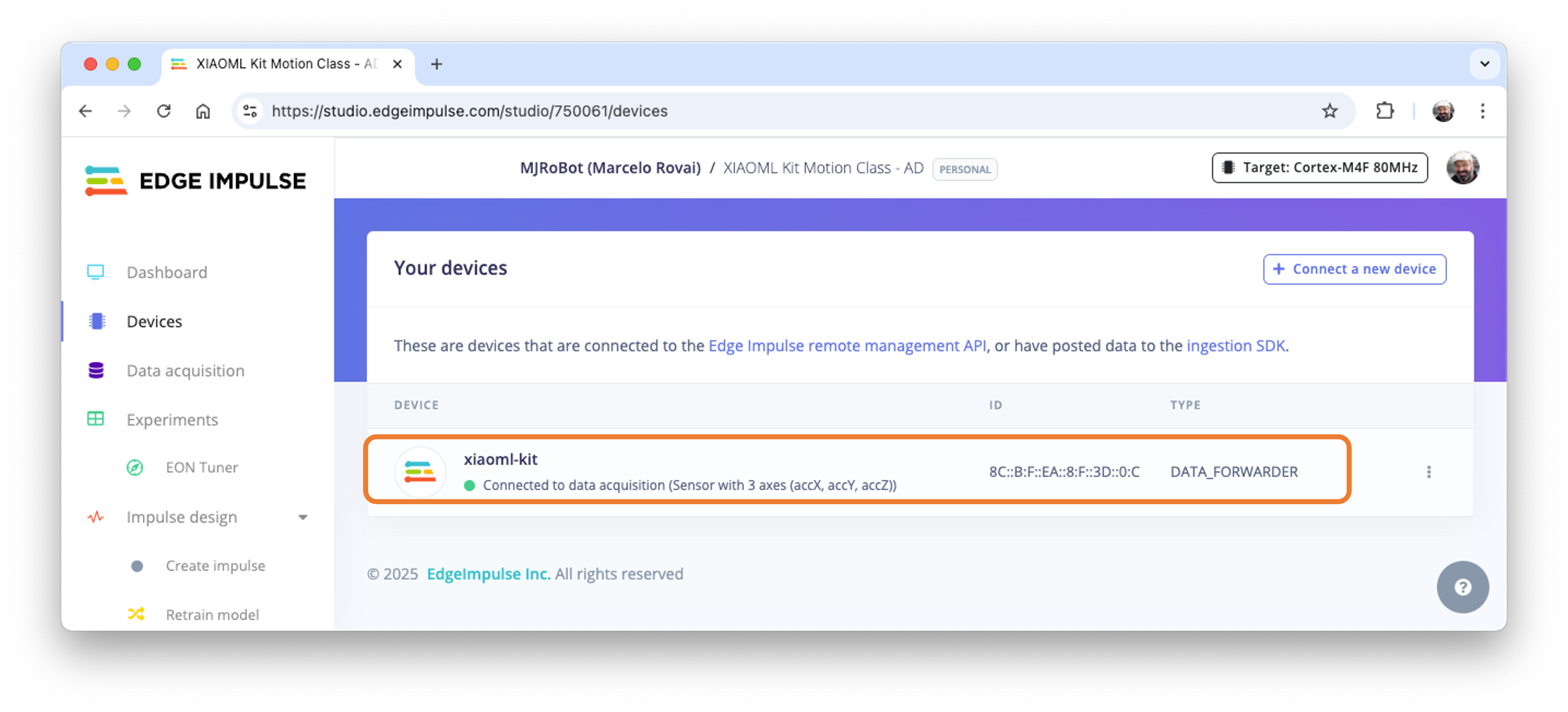
- Go to the Edge Impulse Studio Project. On the
Devicesection is possible to verify if the kit is correctly connected (the dot should be green).
Data Collection at the Studio
As discussed before, we should capture data from all four Transportation Classes. Imagine that you have a container with a built-in accelerometer (In this case, our XIAOML Kit). Now imagine your container is on a boat, facing an angry ocean:
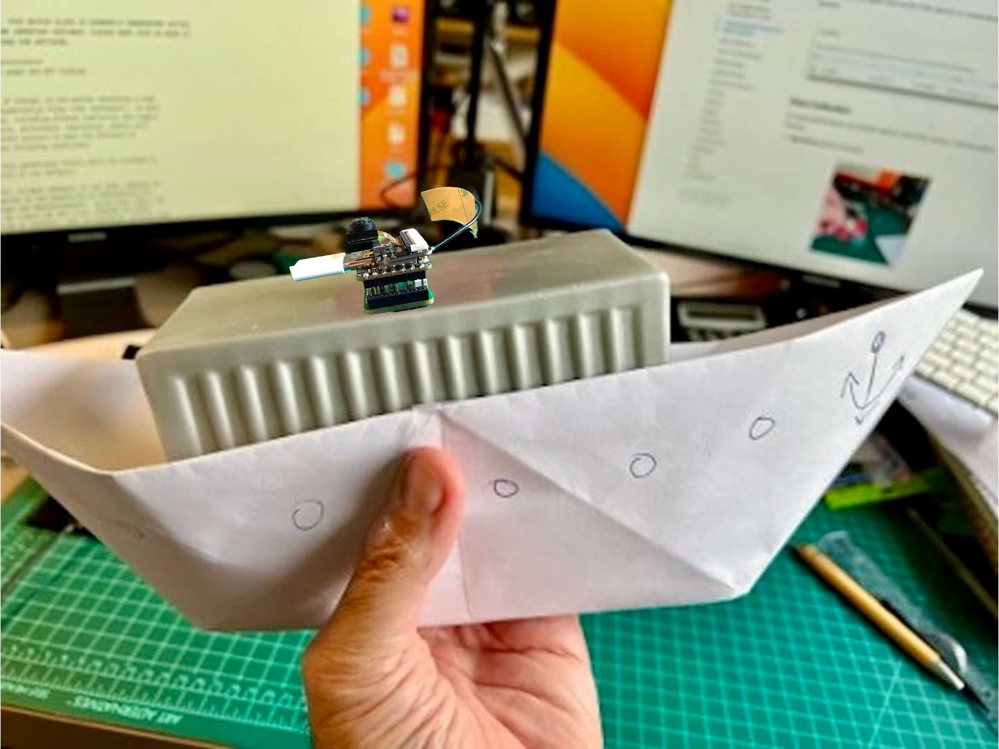
Or in a Truck, travelling on a road, or being moved with a forklift, etc.
Movement Simulation
Maritime Class:
- Hold the kit and simulate boat movement
- Move in all three axes with wave-like, undulating motions
- Include gentle rolling and pitching movements
Terrestrial Class:
- Move the kit horizontally in straight lines (left to right and vice versa)
- Simulate truck/train vibrations with small horizontal shakes
- Occasional gentle bumps and turns
Lift Class:
- Move the kit primarily in vertical directions (up and down)
- Simulate forklift operations: up, pause, down
- Include some short horizontal positioning movements
Idle Class:
- Place the kit on a stable surface
- Minimal to no movement
- Capture environmental vibrations and sensor noise
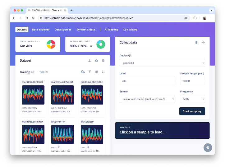
Data Acquisition
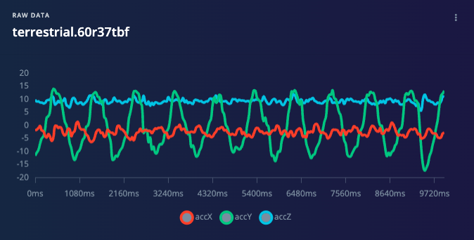
On the Data Acquisition section, you should see that your board [xiaoml-kit] is connected. The sensor is available: [sensor with 3 axes (accX, accY, accZ)] with a sampling frequency of [50 Hz]. The Studio suggests a sample length of [10000] ms (10 s). The last thing left is defining the sample label. Let’s start, for example, with[terrestrial].
Press [Start Sample]and move your kit horizontally (left to right), keeping it in one direction. After 10 seconds, our data will be uploaded to the Studio.
Below is one sample (raw data) of 10 seconds of collected data. It is notable that the ondulatory movement predominantly occurs along the Y-axis (left-right). The other axes are almost stationary (the X-axis is centered around zero, and the Z-axis is centered around 9.8 ms² due to gravity).
You should capture, for example, around 2 minutes (ten to twelve samples of 10 seconds each) for each of the four classes. Using the 3 dots after each sample, select two and move them to the Test set. Alternatively, you can use the Automatic Train/Test Split tool on the Danger Zone of the Dashboard tab. Below, it is possible to see the result datasets:
Data Pre-Processing
The raw data type captured by the accelerometer is a “time series” and should be converted to “tabular data”. We can do this conversion using a sliding window over the sample data. For example, in the below figure,
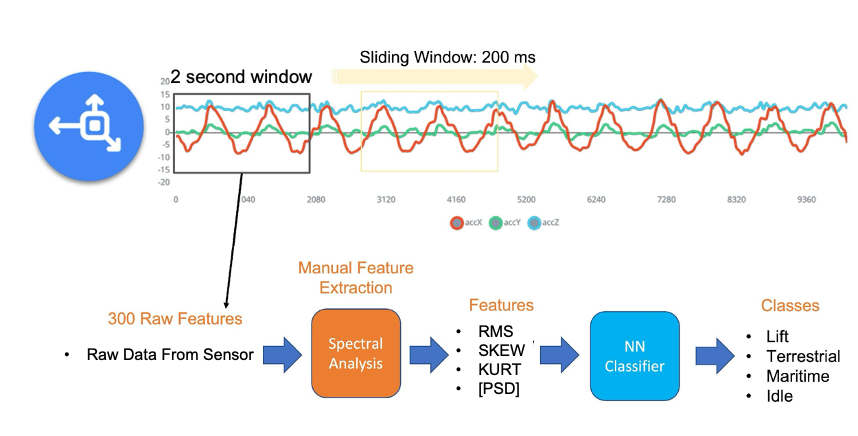
We can see 10 seconds of accelerometer data captured with a sample rate (SR) of 50 Hz. A 2-second window will capture 300 data points (3 axes \(\times\) 2 seconds \(\times\) 50 samples). We will slide this window every 200ms, creating a larger dataset where each instance has 300 raw features.
You should use the best SR for your case, considering Nyquist’s theorem, which states that a periodic signal must be sampled at more than twice the signal’s highest frequency component.
Data preprocessing is a challenging area for embedded machine learning. Still, Edge Impulse helps overcome this with its digital signal processing (DSP) preprocessing step and, more specifically, the Spectral Features.
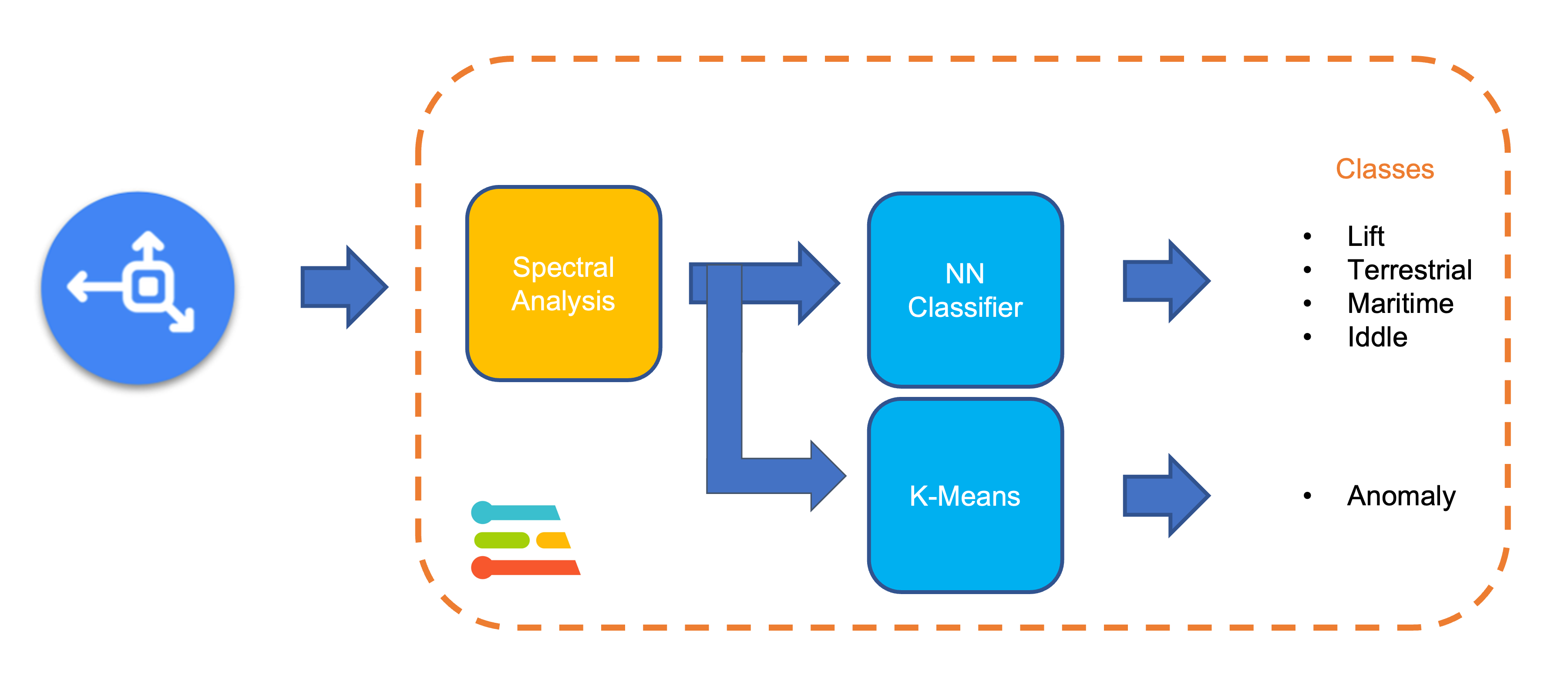
On the Studio, this dataset will be the input of a Spectral Analysis block, which is excellent for analyzing repetitive motion, such as data from accelerometers. This block will perform a DSP (Digital Signal Processing), extracting features such as “FFT” or “Wavelets”. In the most common case, FFT, the Time Domain Statistical features per axis/channel are:
- RMS
- Skewness
- Kurtosis
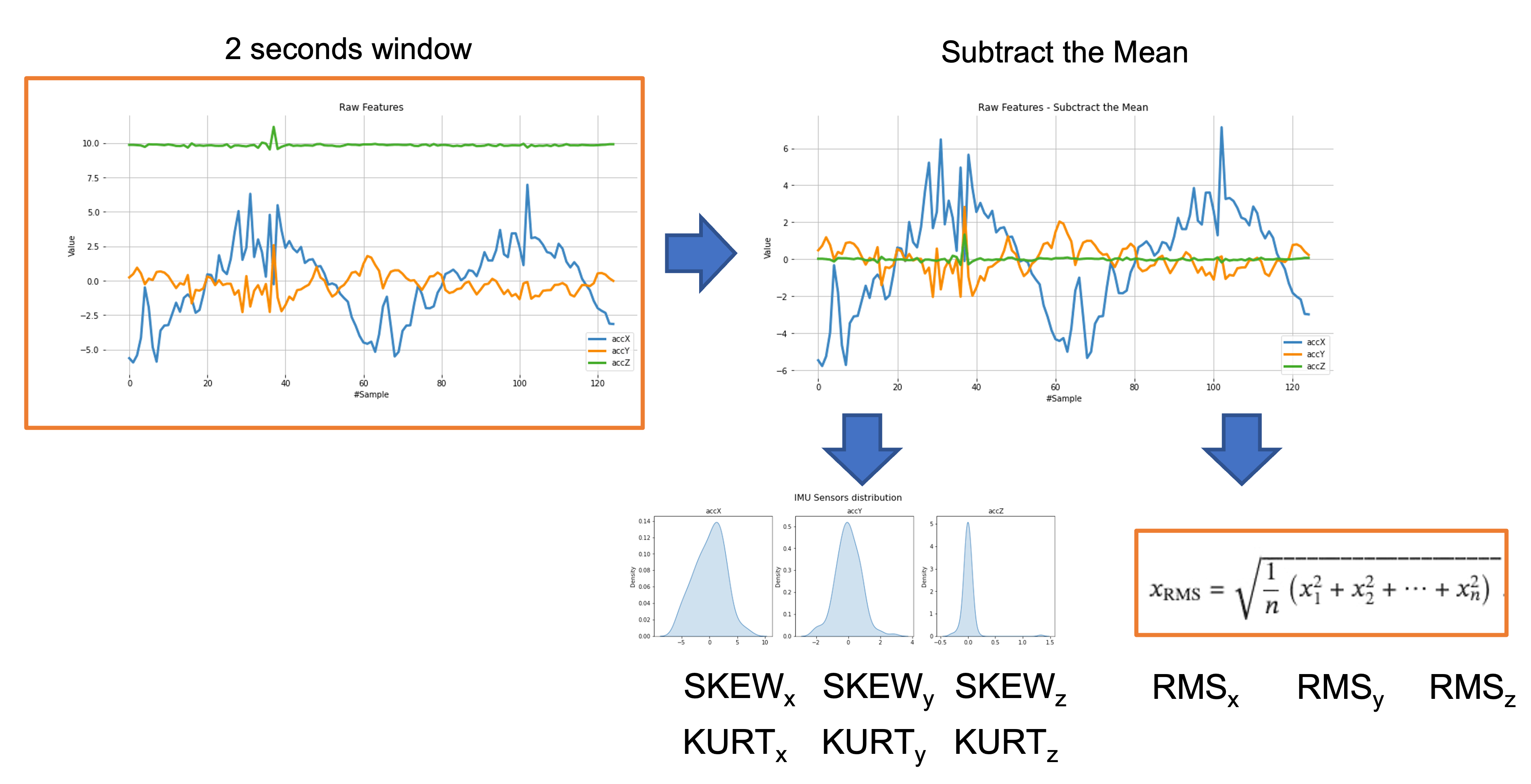
And the Frequency Domain Spectral features per axis/channel are:
- Spectral Power
- Skewness
- Kurtosis
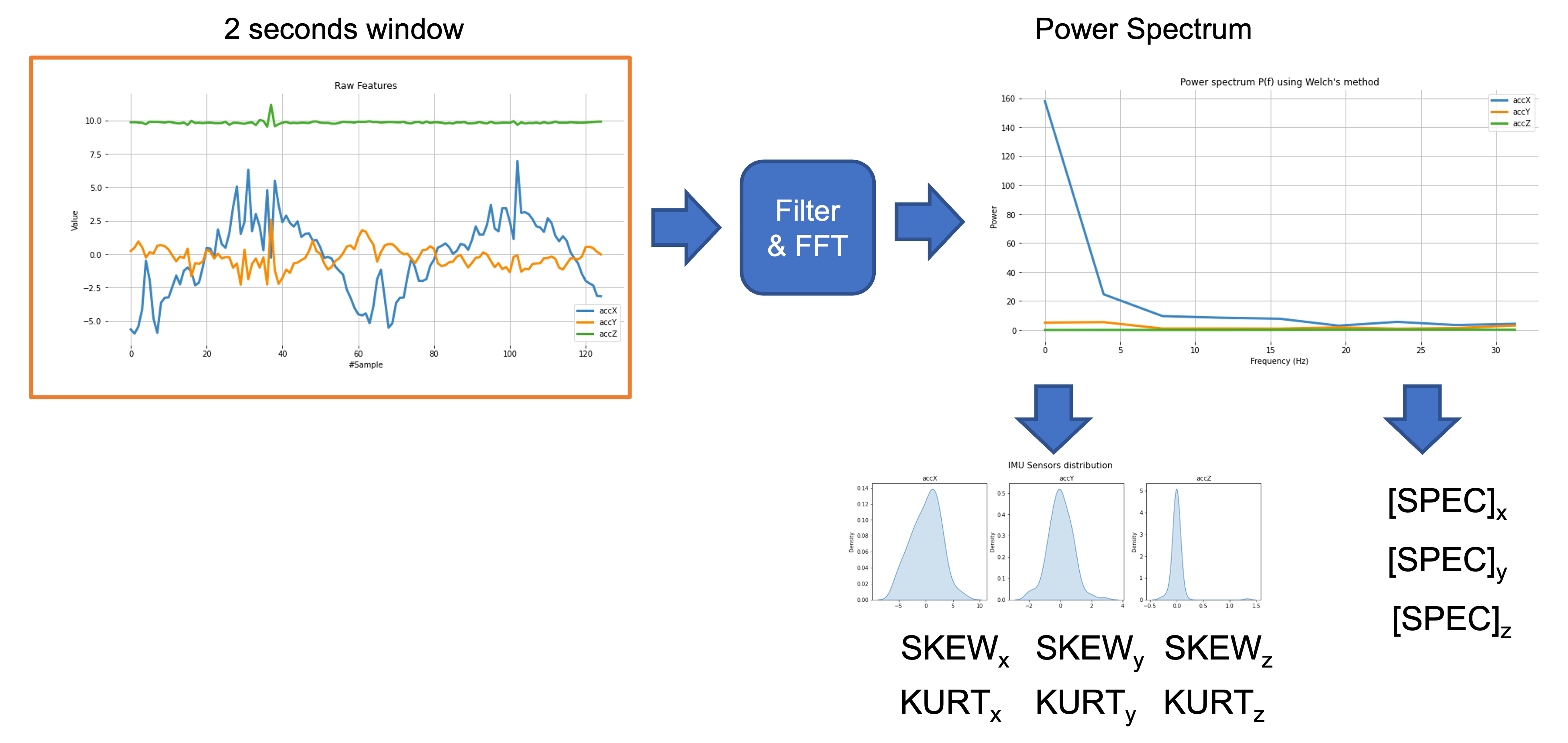
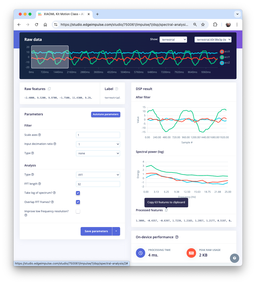
For example, for an FFT length of 32 points, the Spectral Analysis Block’s resulting output will be 21 features per axis (a total of 63 features).
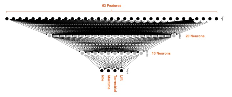
Those 63 features will serve as the input tensor for a Neural Network Classifier and the Anomaly Detection model (K-Means).
You can learn more by digging into the lab DSP Spectral Features
Model Design
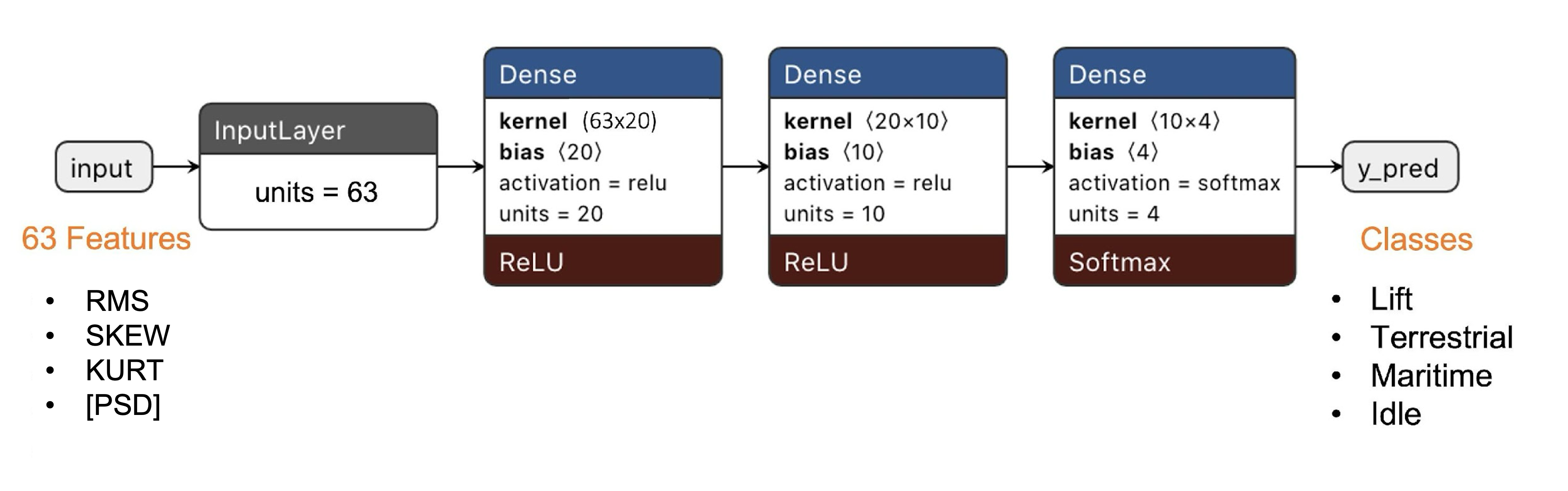
Our classifier will be a Dense Neural Network (DNN) that will have 63 neurons on its input layer, two hidden layers with 20 and 10 neurons, and an output layer with four neurons (one per each class), as shown here:
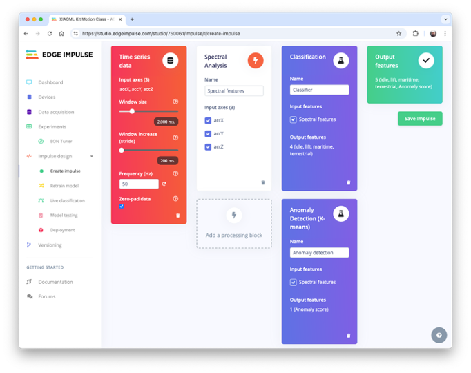
Impulse Design
An impulse takes raw data, uses signal processing to extract features, and then uses a learning block (Dense model) to classify new data.
We also utilize a second model, the K-means, which can be used for Anomaly Detection. If we imagine that we could have our known classes as clusters, any sample that cannot fit into one of these clusters could be an outlier, an anomaly (for example, a container rolling out of a ship on the ocean or being upside down on the floor).
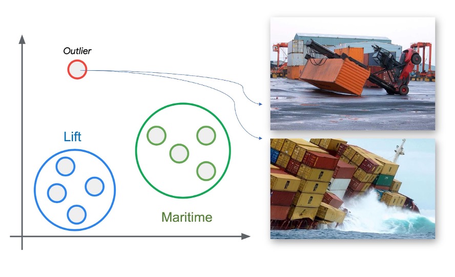
Imagine our XIAOML Kit rolling or moving upside-down, on a movement complement different from the one trained on.
Below the final Impulse design:
Generating features
At this point in our project, we have defined the pre-processing method, and the model has been designed. Now, it is time to have the job done. First, let’s convert the raw data (time-series type) into tabular data. Go to the Spectral Features tab and select [Save Parameters]. Alternatively, instead of using the default values, we can select the [Autotune parameters] button. In this case, the Studio will define new hyperparameters, as the filter design and FFT length, based on the raw data.
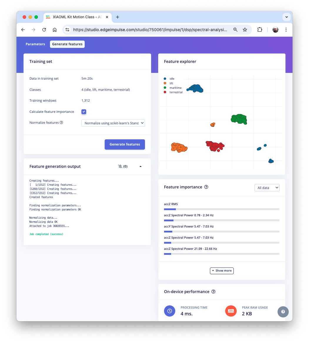
At the top menu, select the Generate features tab, and there, select the options, Calculate feature importance, Normalize features, and press the [Generate features] button. Each 2-second window of data (300 datapoints) will be converted into a single tabular data point with 63 features.
The Feature Explorer will display this data in 2D using UMAP. Uniform Manifold Approximation and Projection (UMAP) is a dimensionality reduction technique that can be used for visualization, similar to t-SNE, but also for general non-linear dimensionality reduction.
The visualization enables one to verify that the classes present an excellent separation, indicating that the classifier should perform well.
Optionally, you can analyze the relative importance of each feature for one class compared with other classes.
Training
Our classifier will be a Dense Neural Network (DNN) that will have 63 neurons on its input layer, two hidden layers with 20 and 10 neurons, and an output layer with four neurons (one per each class), as shown here:
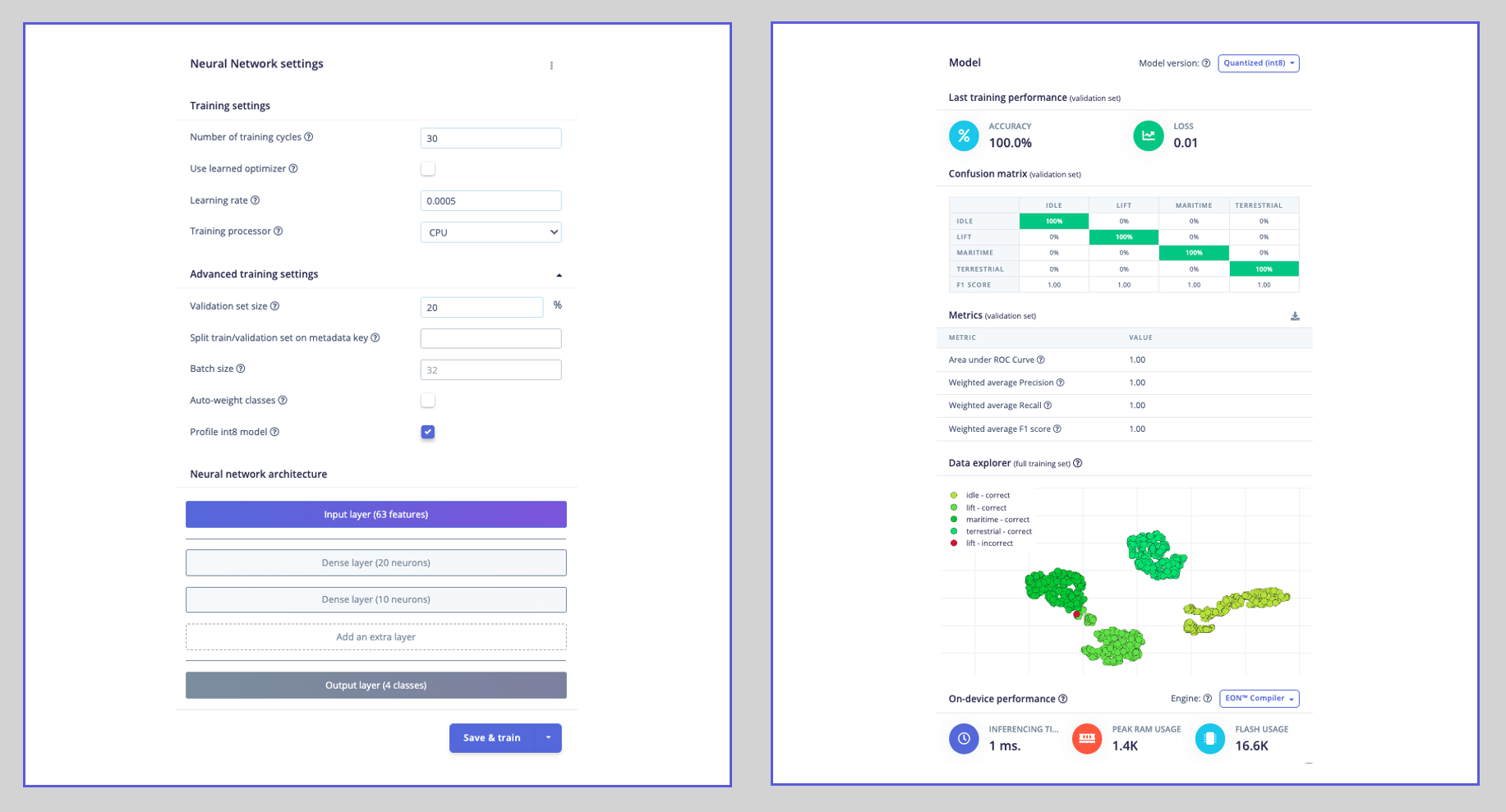
As hyperparameters, we will use a Learning Rate of 0.005 and 20% of the data for validation for 30 epochs. After training, we can see that the accuracy is 100%.
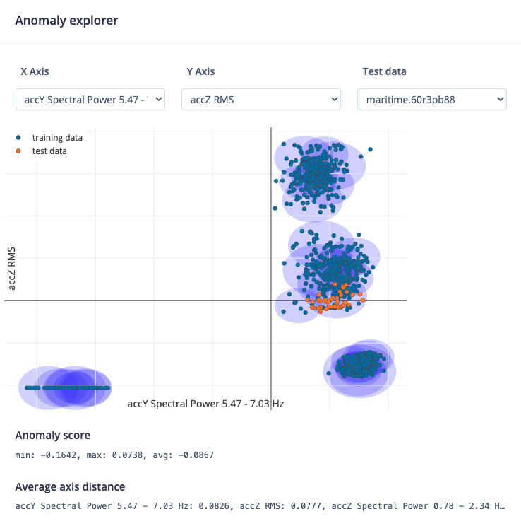
For anomaly detection, we should choose the suggested features that are precisely the most important in feature extraction. The number of clusters will be 32, as suggested by the Studio. After training, we can select some data for testing, such as maritime data. The resulting Anomaly score was min: -0.1642, max: 0.0738, avg: -0.0867.
When changing the data, it is possible to realize that small or negative Anomaly Scores indicate that the data are normal.
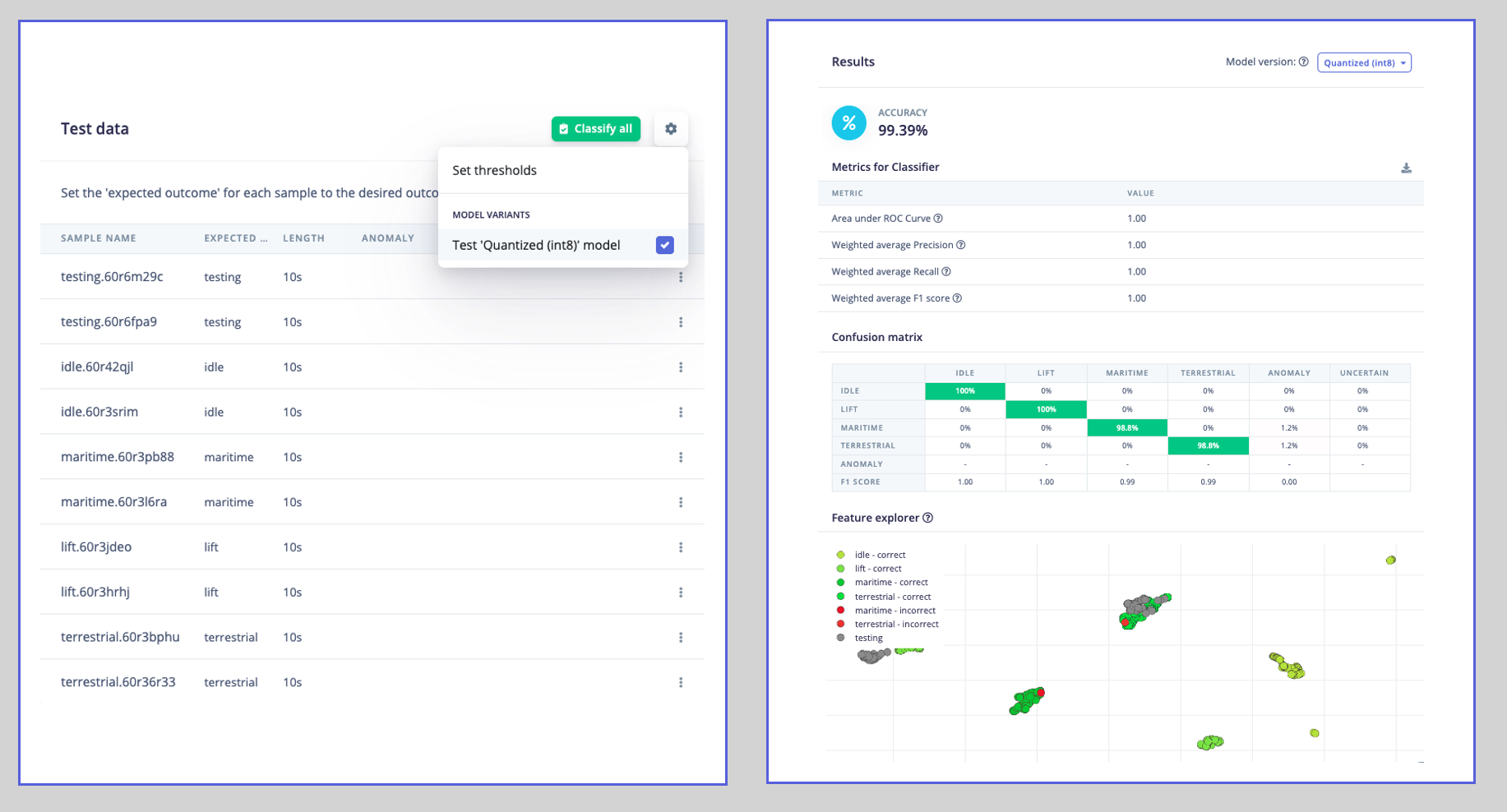
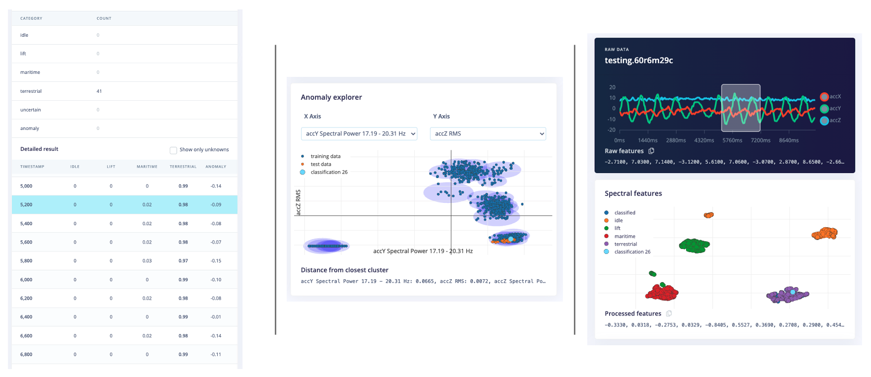
Testing
Using 20% of the data left behind during the data capture phase, we can verify how our model will behave with unknown data; if not 100% (what is expected), the result was very good (8%).
You should also use your kit (which is still connected to the Studio) and perform some Live Classification. For example, let’s test some “terrestrial” movement:
Be aware that here, you will capture real data with your device and upload it to the Studio, where an inference will be made using the trained model (note that the model is not on your device).
Deploy
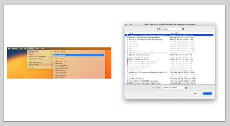
Now it is time for magic! The Studio will package all the needed libraries, preprocessing functions, and trained models, downloading them to your computer. You should select the Arduino Library option, and then, at the bottom, choose Quantized (Int8) and click [Build]. A ZIP file will be created and downloaded to your computer.

On your Arduino IDE, go to the Sketch tab, select the option Add.ZIP Library, and Choose the.zip file downloaded by the Studio:
Inference
Now, it is time for a real test. We will make inferences that are wholly disconnected from the Studio. Let’s change one of the code examples created when you deploy the Arduino Library.
In your Arduino IDE, go to the File/Examples tab and look for your project, and in examples, select nano_ble_sense_accelerometer:
Of course, this is not your board, but we can have the code working with only a few changes.
For example, at the beginning of the code, you have the library related to Arduino Sense IMU:
/* Includes -------------------------------------------- */
#include <XIAOML_Kit_Motion_Class_-_AD_inferencing.h>
#include <Arduino_LSM9DS1.h>
Change the “includes” portion with the code related to the IMU:
#include <XIAOML_Kit_Motion_Class_-_AD_inferencing.h>
#include <LSM6DS3.h>
#include <Wire.h>
Change the Constant Defines
// IMU setup
LSM6DS3 myIMU(I2C_MODE, 0x6A);

// Inference settings
#define CONVERT_G_TO_MS2    9.81f
#define MAX_ACCEPTED_RANGE  2.0f * CONVERT_G_TO_MS2
On the setup function, initiate the IMU:
   // Initialize IMU
    if (myIMU.begin() != 0) {
        Serial.println("ERROR: IMU initialization failed!");
        return;
    }
At the loop function, the buffers buffer[ix], buffer[ix + 1], and buffer[ix + 2] will receive the 3-axis data captured by the accelerometer. In the original code, you have the line:
IMU.readAcceleration(buffer[ix], buffer[ix + 1], buffer[ix + 2]);Change it with this block of code:
// Read IMU data
float x = myIMU.readFloatAccelX();
float y = myIMU.readFloatAccelY();
float z = myIMU.readFloatAccelZ();
You should reorder the following two blocks of code. First, you make the conversion to raw data to “Meters per squared second (m/s2)”, followed by the test regarding the maximum acceptance range (that here is in m/s2, but on Arduino, was in Gs):
  // Convert to m/s²
  buffer[i + 0] = x * CONVERT_G_TO_MS2;
  buffer[i + 1] = y * CONVERT_G_TO_MS2;
  buffer[i + 2] = z * CONVERT_G_TO_MS2;

  // Apply range limiting
  for (int j = 0; j < 3; j++) {
      if (fabs(buffer[i + j]) > MAX_ACCEPTED_RANGE) {
          buffer[i + j] = copysign(MAX_ACCEPTED_RANGE, buffer[i + j]);
      }
  }
And this is enough. We can also adjust how the inference is displayed in the Serial Monitor. You can now upload the complete code below to your device and proceed with the inferences.
// Motion Classification with LSM6DS3TR-C IMU
#include <XIAOML_Kit_Motion_Class_-_AD_inferencing.h>
#include <LSM6DS3.h>
#include <Wire.h>

// IMU setup
LSM6DS3 myIMU(I2C_MODE, 0x6A);

// Inference settings
#define CONVERT_G_TO_MS2    9.81f
#define MAX_ACCEPTED_RANGE  2.0f * CONVERT_G_TO_MS2

static bool debug_nn = false;
static float buffer[EI_CLASSIFIER_DSP_INPUT_FRAME_SIZE] = { 0 };
static float inference_buffer[EI_CLASSIFIER_DSP_INPUT_FRAME_SIZE];

void setup() {
    Serial.begin(115200);
    while (!Serial) delay(10);

    Serial.println("XIAOML Kit - Motion Classification");
    Serial.println("LSM6DS3TR-C IMU Inference");

    // Initialize IMU
    if (myIMU.begin() != 0) {
        Serial.println("ERROR: IMU initialization failed!");
        return;
    }

    Serial.println("✓ IMU initialized");

    if (EI_CLASSIFIER_RAW_SAMPLES_PER_FRAME != 3) {
        Serial.println("ERROR: EI_CLASSIFIER_RAW_SAMPLES_PER_FRAME"
                       "should be 3");
        return;
    }

    Serial.println("✓ Model loaded");
    Serial.println("Starting motion classification...");
}

void loop() {
    ei_printf("\nStarting inferencing in 2 seconds...\n");
    delay(2000);

    ei_printf("Sampling...\n");

    // Clear buffer
    for (size_t i = 0; i < EI_CLASSIFIER_DSP_INPUT_FRAME_SIZE; i++) {
        buffer[i] = 0.0f;
    }

    // Collect accelerometer data
    for (int i = 0; i < EI_CLASSIFIER_DSP_INPUT_FRAME_SIZE; i += 3) {
        uint64_t next_tick = micros() +
          (EI_CLASSIFIER_INTERVAL_MS * 1000);

        // Read IMU data
        float x = myIMU.readFloatAccelX();
        float y = myIMU.readFloatAccelY();
        float z = myIMU.readFloatAccelZ();

        // Convert to m/s²
        buffer[i + 0] = x * CONVERT_G_TO_MS2;
        buffer[i + 1] = y * CONVERT_G_TO_MS2;
        buffer[i + 2] = z * CONVERT_G_TO_MS2;

        // Apply range limiting
        for (int j = 0; j < 3; j++) {
            if (fabs(buffer[i + j]) > MAX_ACCEPTED_RANGE) {
                buffer[i + j] = copysign(MAX_ACCEPTED_RANGE,
                                         buffer[i + j]);
            }
        }

        delayMicroseconds(next_tick - micros());
    }

    // Copy to inference buffer
    for (int i = 0; i < EI_CLASSIFIER_DSP_INPUT_FRAME_SIZE; i++) {
        inference_buffer[i] = buffer[i];
    }

    // Create signal from buffer
    signal_t signal;
    int err = numpy::signal_from_buffer(inference_buffer,
              EI_CLASSIFIER_DSP_INPUT_FRAME_SIZE, &signal);
    if (err != 0) {
        ei_printf("ERROR: Failed to create signal from buffer (%d)\n",
                  err);
        return;
    }

    // Run the classifier
    ei_impulse_result_t result = { 0 };
    err = run_classifier(&signal, &result, debug_nn);
    if (err != EI_IMPULSE_OK) {
        ei_printf("ERROR: Failed to run classifier (%d)\n", err);
        return;
    }

    // Print predictions
    ei_printf("Predictions (DSP: %d ms, Classification: %d ms, "
              "Anomaly: %d ms):\n",
        result.timing.dsp, result.timing.classification, result.timing.anomaly);

    for (size_t ix = 0; ix < EI_CLASSIFIER_LABEL_COUNT; ix++) {
        ei_printf("    %s: %.5f\n", result.classification[ix].label,
                  result.classification[ix].value);
    }

    // Print anomaly score
#if EI_CLASSIFIER_HAS_ANOMALY == 1
    ei_printf("Anomaly score: %.3f\n", result.anomaly);
#endif

    // Determine prediction
    float max_confidence = 0.0;
    String predicted_class = "unknown";

    for (size_t ix = 0; ix < EI_CLASSIFIER_LABEL_COUNT; ix++) {
        if (result.classification[ix].value > max_confidence) {
            max_confidence = result.classification[ix].value;
            predicted_class = String(result.classification[ix].label);
        }
    }

    // Display result with confidence threshold
    if (max_confidence > 0.6) {
        ei_printf("\n🎯 PREDICTION: %s (%.1f%% confidence)\n",
                 predicted_class.c_str(), max_confidence * 100);
    } else {
        ei_printf("\n❓ UNCERTAIN: Highest confidence is %s (%.1f%%)\n",
                 predicted_class.c_str(), max_confidence * 100);
    }

    // Check for anomaly
#if EI_CLASSIFIER_HAS_ANOMALY == 1
    if (result.anomaly > 0.5) {
        ei_printf("⚠️ ANOMALY DETECTED! Score: %.3f\n", result.anomaly);
    }
#endif

    delay(1000);
}

void ei_printf(const char *format, ...) {
    static char print_buf[1024] = { 0 };
    va_list args;
    va_start(args, format);
    int r = vsnprintf(print_buf, sizeof(print_buf), format, args);
    va_end(args);
    if (r > 0) {
        Serial.write(print_buf);
    }
}
The complete code is available on the Lab’s GitHub.
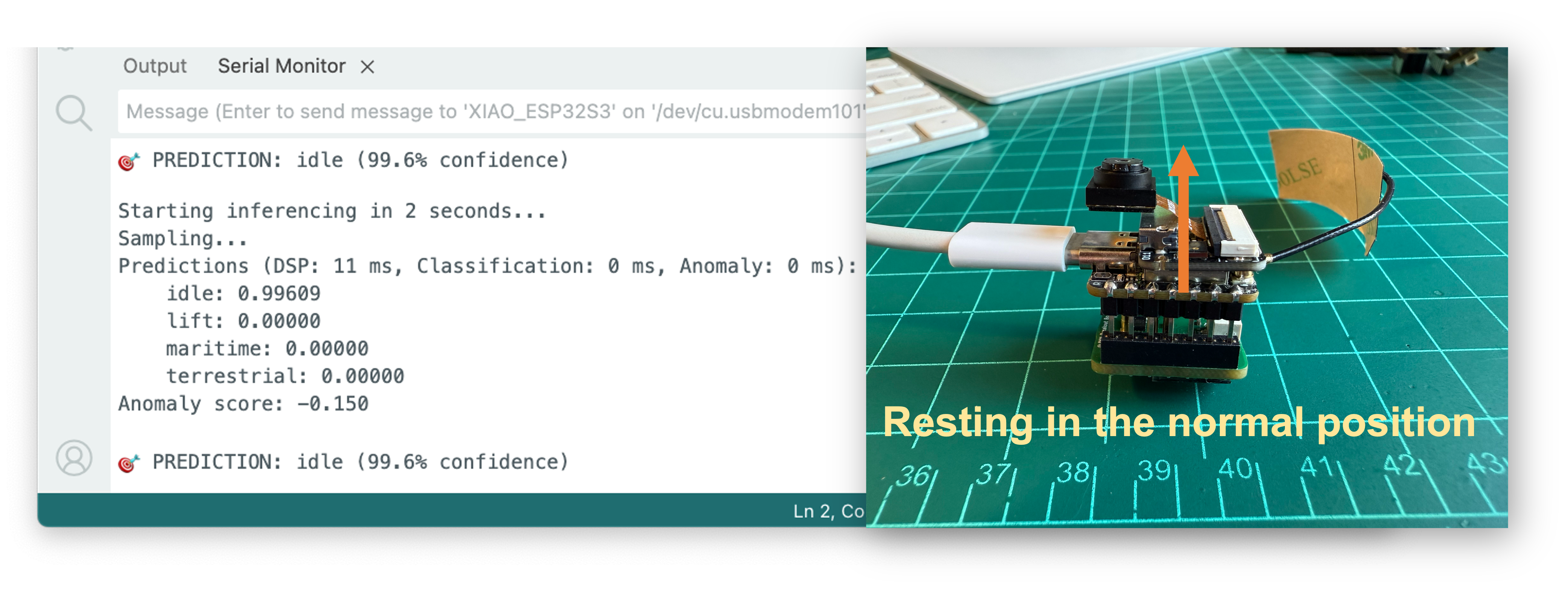
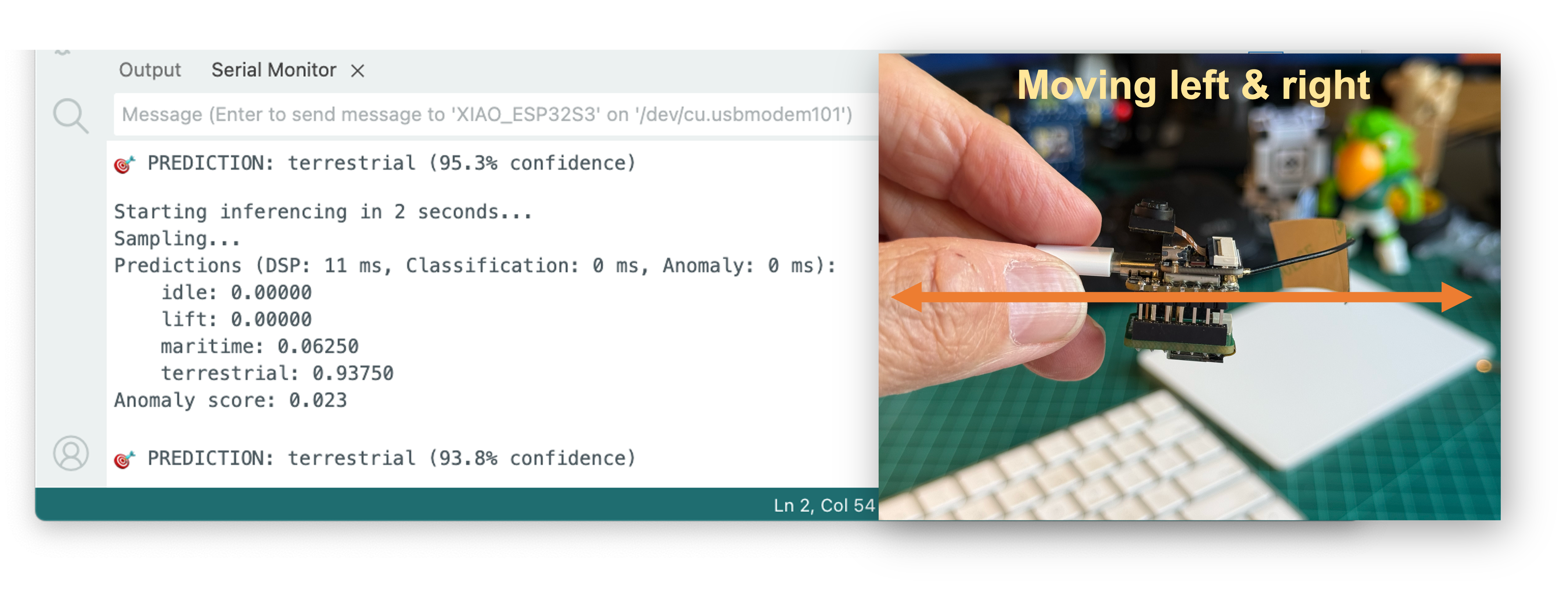
Now you should try your movements, seeing the result of the inference of each class on the images:

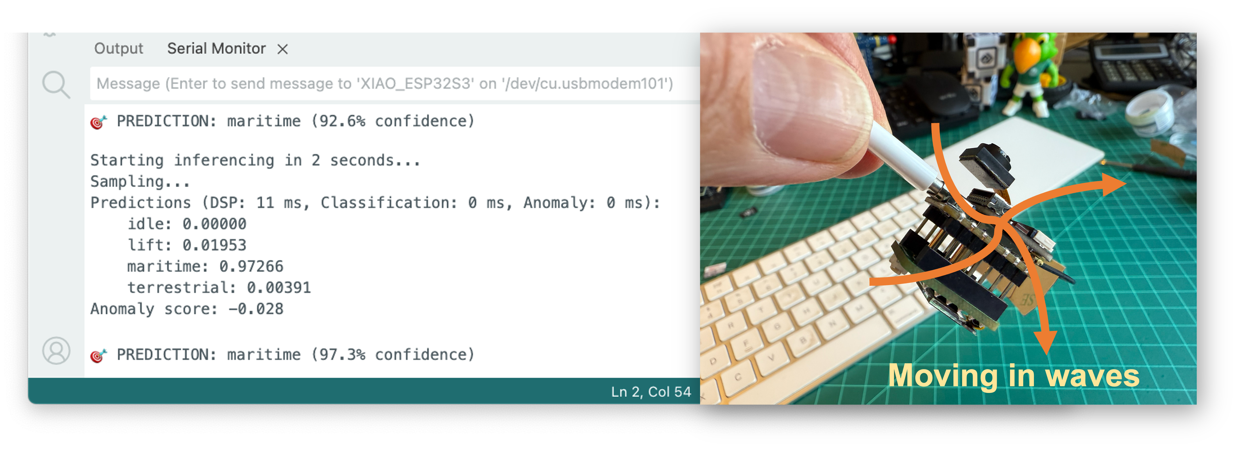
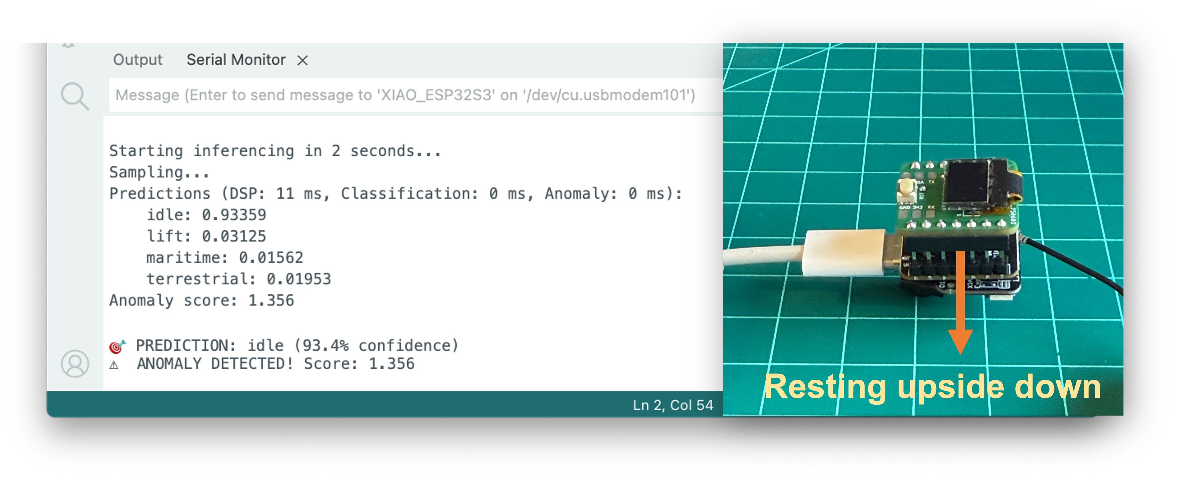
And, of course, some “anomaly”, for example, putting the XIAO upside-down. The anomaly score will be over 0.5:
Post-Prossessing
Now that we know the model is working, we suggest modifying the code to see the result with the Kit completely offline (disconnected from the PC and powered by a battery, a power bank, or an independent 5V power supply).
The idea is that if a specific movement is detected, a corresponding message will appear on the OLED display.
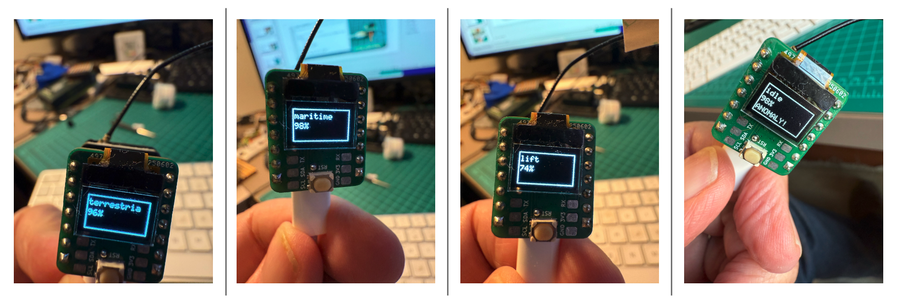
The modified inference code to have the OLED display is available on the Lab’s GitHub.
Summary
This lab demonstrated how to build a complete motion classification system using the XIAOML Kit’s built-in LSM6DS3TR-C IMU sensor. Key achievements include:
Technical Implementation:
- Utilized the integrated 6-axis IMU for motion sensing
- Collected labeled training data for four transportation scenarios
- Implemented spectral feature extraction for time-series analysis
- Deployed a neural network classifier optimized for microcontroller inference
- Added anomaly detection for identifying unusual movements
Machine Learning Pipeline:
- Data collection directly from embedded sensors
- Feature engineering using frequency domain analysis
- Model training and optimization in Edge Impulse
- Real-time inference on resource-constrained hardware
- Performance monitoring and validation
Practical Applications: The techniques learned apply directly to real-world scenarios, including:
- Asset tracking and logistics monitoring
- Predictive maintenance for machinery
- Human activity recognition
- Vehicle and equipment monitoring
- IoT sensor networks for smart cities
Key Learnings:
- Working with IMU coordinate systems and sensor fusion
- Balancing model accuracy with inference speed on edge devices
- Implementing robust data collection and preprocessing pipelines
- Deploying machine learning models to embedded systems
- Integrating multiple sensors (IMU + display) for complete solutions
The integration of motion classification with the XIAOML Kit demonstrates how modern embedded systems can perform sophisticated AI tasks locally, enabling real-time decision-making without reliance on the cloud. This approach is fundamental to the future of edge AI in industrial IoT, autonomous systems, and smart device applications.
Resources
- XIAOML KIT Code
- DSP Spectral Features
- Edge Impulse Project
- Edge Impulse Spectral Features Block Colab Notebook
- Edge Impulse Documentation
- Edge Impulse Spectral Features
- Seeed Studio LSM6DS3 Library